Introduction

Background to the study

Agricultural development is one of the most powerful tools to end extreme poverty, boost shared prosperity and feed a projected 9.7 billion people by 2050.  Growth in the agriculture sector is two to four times more effective in raising incomes among the poorest compared to other sectors. 2016 analyses found that 65% of poor working adults made a living through agriculture. Agriculture is also crucial to economic growth: in 2014, it accounted for one-third of global gross-domestic product (GDP) [1]. Agriculture is the science or practice of farming, including cultivation of the soil for the growing of crops and the rearing of animals to provide food, wool, and other products while agricultural productivity is increase in per capita output of agricultural produce (Stamp 1970). To meet the needs of a world population expected to reach nine billion by 2050, agricultural production will need to increase by at least 60 percent [2]. Due to its relative importance and future gains, it is known to be a major source of raw materials for processing industries in the manufacturing of finished goods and services. It produces about 80% of all manufacturing industries’ raw materials used in the production of finished goods in most economies of the world. For many years, productivity has been a key issue of agricultural development strategies because of its impact on economic growth and development. It is also a known fact that the easiest means through which mankind can get out of poverty to a condition of relative material affluence is by increasing agricultural productivity. Productivity improvements create the wealth that can be used to meet the needs of the future.

Problem Statement: The development of agriculture in Nigeria has been slow despite various agricultural policies and programmes formulated by successive administration in the country. In fact, the government recognized the unhealthy condition of Nigerian agricultural sector since 1970, and has formulated and introduced a number of programmes and strategies aimed at remedying this situation. These measures included the setting up of large-scale mechanized farms by state and federal government, introduction of scheme such as the River Basin Development Authority. Other measures include, National Accelerated Food Production (NAFP), Operation Feed the Nation (OFN), Green Revolution (GRP) and the Directorate for Food, Roads and Rural Infrastructure, the New Nigerian Agricultural Policy etc. [3]. In addition to these measures, financial measures such as the establishment of agricultural credit scheme were introduced by successive governments. Inspite of these measures, the development of the agricultural sector has been slow and the impact of this sector on economic growth and development has been minimal. In fact, the former Minister of Agriculture, Dr. Akinwunmi Adesina once lamented that the import bill for food in Nigeria is exceptionally high and it is growing at an unsustainable rate of 11% per annum. Ironically, Nigeria is importing what it can produce in abundance. This trend is hurting Nigerian farmers and displacing local production [4]. In the same vein, Senator Ibikunle Amosun once lamented the high rate of importation of food in Nigeria, describing it as a shame that the giant of Africa imports what it eats [5]. It is in view of the foregoing that the present paper intends to examine the effect of agricultural inputs on agricultural productivity in Nigeria between 1990 to 2016, using an econometric approach of Ordinary Least Squares Regression.

Study Objectives: Specifically, the study is designed to achieve the following objectives in addition to the broad objective earlier stated.

(i) Examine the effect of Agricultural machinery (tractors) on agricultural productivity in Nigeria;

(ii) Determine the impact of Agricultural credit (loans) on agricultural productivity in Nigeria;

(iii)Examine the causality effect of government expenditure on agriculture on agricultural productivity.

Research Hypothesis: The study shall adopt statistical testing criteria to examine the veracity of the following hypothesis:

Ho1: Agricultural machinery has no significant effect on agricultural productivity in Nigeria;

Ho2: Agricultural credit has no significant impact on agricultural productivity in Nigeria;

Ho3: Government expenditure on Agriculture has no causality effect on agricultural productivity in Nigeria.

Justification for the study: The study is justified because it will provide an insight into how effective both fiscal and monetary instruments designed by the Central Bank of Nigeria and the Nigerian government helped in achieving the overall objectives of the nation’s agricultural policy which is first and foremost tailored towards achieving food security and exportable surplus for enhanced economic growth and development. Furthermore, the study is expected to serve as a reference material for future research as well as guide government in its future policy designs towards achieving country-wide expected goals.

The remainder of this study is sectionalized as follows: Part two is dedicated to theoretical and empirical review. In part three, the data and methodology adopted for the study is discussed. Part four presents the empirical findings, while part five provides the conclusion and policy recommendations of the study.

Literature Review

Agricultural productivity

According to Fulginiti and Perrin [6], as cited in Amire and Arigbede [2], agricultural productivity refers to the output produced by a given level of inputs in the agricultural sector of a given economy. More formally, it can be defined as “the ratio of value of total farms outputs to the value of total inputs used in farm production” [7], as cited in [8]. Put differently, agricultural productivity is measured as the ration of final output, in appropriate units to some measure of inputs.

An overview of agricultural policies in Nigeria

In the view of Nwagbo [9], agricultural policy-making in Nigeria has been through changes over time. During each phase, the characteristics of policy have reflected the roles expected of the sector and the relative endowment of resources. Institutions were created while others were disbanded depending on the exigencies of the time. Hence the marketing Boards gave way to commodity boards and production companies; the River Basin development Authorities have been modified to meet changing objectives; small-scale irrigation schemes are receiving more attention than the earlier large versions; agricultural extension by the State Ministries of Agriculture has given way to extension by the Agricultural Development Project (ADP). Other measures include, National Accelerated Food Production (NAFP), Operation Feed the Nation (OFN), Green Revolution (GRP) and the Directorate for Food, Roads and Rural Infrastructure and finally, the New Nigerian Agricultural Policy. The first national policy on agriculture was adopted in 1988 and was expected to remain valid for about fifteen years, that is, up to year 2000. Nigeria’s agricultural policy is the synthesis of the framework and action plans of government designed to achieve overall agricultural growth and development. The policy aims at the attainment of self-sustaining growth in all the sub-sectors of agriculture and the structural transformation necessary for the overall socio-economic development of the country as well as the improvement in the quality of life of Nigerians.

According to ARCN (2016) [10], the broad policy objectives Include:

• Attainment of self-sufficiency in basic food commodities With particular reference to those which consume considerable shares of Nigeria’s foreign exchange and for which the country has comparative advantage in local production;

• Increase in production of agricultural raw materials to meet the growth of an expanding industrial sector;

• Increase in production and processing of exportable Commodities with a view to increasing their foreign exchange earning capacity and further diversifying the country’s export base and sources of foreign exchange earnings;

• Modernization of agricultural production, processing, Storage and distribution through the infusion of improved technologies and management so that agriculture can be more responsive to the demands of other sectors of that Nigerian economy;

• Creation of more agricultural and rural employment Opportunities to increase the income of farmers and rural dwellers and to productively absorb an increasing labour force in the nation;

• Protection and improvement of agricultural land resources and preservation of the environment for sustainable agricultural production;

• Establishment of appropriate institutions and creation of administrative organs to facilitate the integrated development and realization of the country’s agricultural potentials.

Theoretical framework

The theoretical framework of this study is built on the Cobb-Douglas production function. This theoretical model was applied in extant literature including Ekwere [11]. In economics, the Cobb-Douglas functional form of production function is widely used to represent the relationship of an output to input. It was proposed by Knut (1926) and tested against statistical evidence by Charles Cobb and Paul Douglas in. In 1928, Charles Cobb and Paul Douglas [12], published a study in which they modeled the growth of the American economy during the period 1899 to 1922. They considered a simplified view of the economy in which production output was determined by the amount of labour involved and the amount of capital invested. While there are many other factors affecting economic performance, their model proved to be remarkably accurate. The function they used to model production was of the form:

P(L,K) = bLα Kβ

Where:

P = Total production (the monetary value of all goods produced in a year);

L = Labor input (the total number of person-hours worked in a year);

K = Capital input (the monetary worth of all machinery, equipment, and buildings);

b = Total factor productivity; α and β are the output elasticities of labour and capital, respectively. These values are constants determined by available technology. Output elasticity measures the responsiveness of output to a change in levels of either labour or capital used in production, ceteris paribus.

In agricultural production, efficient allocation of farm resources helps farmers to attain their objectives. It avails farmers the opportunity of improving their productivity and income. At the microeconomic level efficient allocation of farm resources (farmland, credit facilities, fertilizer, tractors and labour, among others) help farmers to contribute to food production, employment creation, industrial raw materials and export product for foreign exchange earnings. According to Olayide and Heady [7], agricultural productivity is synonymous with resource productivity which is the ratio of total output to the resource/inputs being considered. According to Olujenyo (2008), the production function could be expressed in different functional forms such as Cobb Douglas, linear, quadratic, polynomials and square root polynomials, semilog and exponential functions. However, the Cobb Douglas functional form is commonly used for its simplicity and flexibility coupled with the empirical support it has received from data for various industries and countries.

Materials and Methods

This study adopts a non-experimental research design approach. The data used were obtained from secondary sources and therefore, no sampling was done neither was any sampling technique adopted in the process of research.

Sources of data collection

The data for this study were secondary in nature and sourced from the publication of World Bank Database and Central Bank of Nigeria (CBN) [13], statistical bulletin for various issues. The data spans the period 1990 to 2016 (26 years). The data from this period present a considerable degree of freedom that is necessary to capture the effect of explanatory variables on the dependent variables. Furthermore, data sourced from the World Bank can be reliable because many studies have employed the data published by this institution for econometric purposes due to its reliability.

Variables adopted for the study

Variables adopted for the study are Ag-output (proxy for agricultural productivity) used as dependent variable to be regressed against Ag-Machine (proxy for Agricultural machinery, tractors per 100sq.km of arable land), Ag-Exp (proxy for government expenditure on agriculture) and gross domestic product as independent variables respectively. Gross Domestic Product is included as a control variable to avoid the challenge of variable omission and model misspecification.

Method of data analysis

The method of data analysis include first and foremost unit root test using Augmented Dickey-Fuller (ADF); a test for long-run relationship (Johansen cointegration), Granger causality test and then the ordinary least square (OLS) multiple regression method to determine the effect of the independent variables in the model on the dependent variable. The study made use of E-views 8.0, econometric software for the analysis.

Unit root test: To study the stationarity properties of time series, the Augmented Dickey–Fuller test (ADF) (Dickey & Fuller, 1981) is employed in this study. The test involves estimating the regression.

The model for the ADF unit root framework is as follows:

ΔX_t = α_t1+ pt + βX_t-1 +${\displaystyle \sum _{i=1}^{k-1}}$ γ_iΔX_t-1 + ε_t ……. Eq 3.1

In the above equation, α is the constant and ρ is the coefficient of time trend. X is the variable under consideration. In this study, the variables include log(FDI), log(GDP-pc), log(INVT), and log(MAN). Δ is the first-difference operator; t is a time trend; and εt is a stationary random error. The test for a unit root is conducted on the coefficient of Xt-1 in the above regression. If the coefficient, β, is found to be significantly different from zero (β ≠ 0), the null hypothesis that the variable X contains a unit root problem is rejected, implying that the variable does not have a unit root. The optimal lag length is also determined in the ADF regression and is selected using Akaike information criterion (AIC).

Johansen cointegration test: This paper attempts to use the Johansen maximum likelihood cointegration test (Johansen, 1988) to determine long-run relationships among the variables being investigated. In examining causality, the Granger causality analysis is also performed. In order to obtain good results from the test, selecting the optimal lag length is so important. The Johansen cointegration framework takes its starting point in the vector autoregressive (VAR) model of order p given by:

yt = A1yt-1 + …+ Apyt-p + βxt + εt ……. Eq 3.2

where yt is a vector of endogenous variables and A represents the autoregressive matrices. xt is the deterministic vector and B represents the parameter matrices. εt is a vector of innovations and p is the lag length. The VAR can be re-written as:

Δyt = Πyt-1 +${\displaystyle \sum _{i=1}^{p-1}}$ ΓiΔyt-1 + βXt + εt ……. Eq 3.3

where Π = Σ Ai – I and ΓI Σ A I=1 j=i+1j

The matrix Π contains the information regarding the long-run coefficients of the yt variables in the vector. If all the endogenous variables in yt are cointegrated at order one, the cointegrating rank, r, is given by the rank of Π = αβ, where the elements of _ are known as the corresponding adjustment of coefficient in the VEC model and β represents the matrix of parameters of the cointegrating vector. To indicate the number of cointegrating rank, two likelihood ratio (LR) test statistics, namely the trace and the maximum Eigen value tests (Johansen, 1988), are used to determine the number of cointegrating vectors. The two tests are defined as:

ƛtrace = −T Σi=r+1 log(1-ƛ_i) and ƛmax = -Tlog(1- ƛ_i+1), …. Eq 3.4

where ƛ_i denotes the estimated values of the characteristic roots obtained from the estimated Π, and T is the number of observations. The first statistic test tests H₀ that the number of cointegrating vector is less than or equal to r against the alternative hypothesis of k cointegrating relations, where k is the number of endogenous variables, for r = 0,1, … , k−1. The alternative of k cointegrating relations corresponds to the case where none of the series has a unit root. The second test tests the null that the number of cointegrating vectors is r, against the alternative hypothesis of 1 + r cointegrating vectors.

Granger causality based on the vector error correction model: In order to identify the long-run relationship among the series under study, the Johansen co-integration test must be done. However, the test does not indicate anything about the direction of causality among the variables in the system; therefore, the Granger causality analysis must be done. If the series are co-integrated, the VECM-based Granger causality analysis is an appropriate technique used to determine the long-run and the short-run relationships (Engle & Granger, 1987) based on the following forms:

Causality Model: y = [log(Ag-output), log(Ag-Exp]

Δlog(Ag-output)_t = β_1,t +${\displaystyle \sum _{i=1}^{n-1}}$ β11j, Δlog(Ag-output)t-j +${\displaystyle \sum _{i=1}^{n-1}}$ β11j, Δlog(Ag-Exp)t-j + δ1EC + ε1t Eqtn 3.5

Δlog(Ag-Exp)t = β2,t +${\displaystyle \sum _{i=1}^{n-1}}$ β21,j, Δlog(Ag-Exp)t-j +${\displaystyle \sum _{i=1}^{n-1}}$ β22,j Δlog(Ag-Output)t-j + δ2EC + ε2t Eqtn 3.6

The coefficients of the ECt−1 term indicate causality in the long run and the joint F test of the coefficients of the first-differenced independent variables confirms short-run causality. Δ denotes first-difference operator. μ1t and μ2t are the stationary disturbance terms for the equations. n is the order of the VAR, which is translated into lag of n−1 in the error correction mechanism. δ1 and δ2 denote the coefficients of long-run Granger causality for equations (3.5) and (3.6), respectively. In this paper, the short-run causality is determined through the error correction based on vector error correction model.

Ordinary Least Square (OLS): To examine the effect of agricultural inputs on agricultural productivity in Nigeria using the Ordinary Least Squares (OLS) technique the following model is specified. The model for this study is specified in both linear and non-linear relationship as follows:

The functional form of the model is specified hereunder

Ag-output = f(Ag-Machine, Ag-Credit, Ag-Exp, Gdp) .... Eq 3.7

The mathematical form of the model is specified below

Ag-output = f(Ag-Machine + Ag-Credit + Ag-Exp + Gdp)... Eq 3.8

The statistical form of the model is

Ag-output = β_o + β₁(Ag-Machine) + β₂(Ag-Credit) + β₃(Ag-Exp) + β₄(Gdp) … Eq 3.9

In order to capture the stochastic term µt of the variables, the explicit form of the models is given in econometric form below:

Ag-output = β_o + β₁(Ag-Machine) + β₂(Ag-Credit) + β₃(Ag-Exp) + β₄(Gdp) + µt ….. Eq 3.10

The estimated models are further transformed into log-linear form. This is aimed at reducing the problem of multi-collinearity among the variables in the models. Thus the log-linear models are specified as shown below:

LnAg-output = β_o+β₁(LnAg-Machine) + β₂(LnAg-Credit) + β₃(LnAg-Exp) + β₄(LnGdp) + µt … Eq 3.11

β₁> _o, β₂ > 0, β₃ > 0, β₄ > 0, β₅ > 0

Where,

Ag-output = Agricultural Productivity

Ag-Machine = Agricultural machinery, tractors per 100 sq. km of arable land),

Ag-Credit = Agric credit (proxied by credit to the private sector)

Ag-Exp = Government Expenditure on Agriculture

Gdp = Gross Domestic Product

µ_i = Stochastic or error term

Ln = Natural logarithms

β_o = Intercept parameter

β₁ - β₁ = Slope parameters

Economic A priori

A priori, it is expected that the independent variables agricultural machineries, agricultural credit, government expenditure on agriculture and gross domestic product should be positively related to the dependent variable (agricultural productivity), all things being equal.

Results and Discussion

Data description and sources

This paper used secondary data (time series data). Empirical investigation was carried out on the basis of the sample covering the period 1990 to 2016. Data for the study was sourced from the database of World Bank and Central Bank of Nigeria Statistical Bulletin (2016) respectively. The variables studied include Ag-Output (proxy for agricultural productivity in Nigeria), Ag-Machine (Agricultural machinery, tractors per 100 sq. km of arable land), Ag-Credit ((proxied by credit to the private sector), Ag-Exp (proxy for Government Expenditure on Agriculture) and GDP (proxy for economic growth in Nigeria). Below is the data presentation (Table 1).

1. 

   Table Options

   • View in workspace

   
   

   Table 1:

   Data Presentation on Ag-Output, Ag-Machine, Ag-Credit, Ag-Exp, GDP (1990-2016).
   
   

   ×

   Table 1: Data Presentation on Ag-Output, Ag-Machine, Ag-Credit, Ag-Exp, GDP (1990-2016).
   Year	Ag-Output	Ag-Machine	Ag-Credit	Ag-Exp	GDP
   1990	9,213,962,202.32	13900	8.692986	0.26	2.82E+11
   1991	8,113,215,683.01	14450	8.951905	0.21	3.29E+11
   1992	7,660,938,111.43	15000	13.32934	0.46	5.55E+11
   1993	5,117,718,984.55	15550	12.19857	1.80	7.15E+11
   1994	6,680,276,587.61	16100	14.9541	1.18	9.46E+11
   1995	8,809,079,448.55	16650	10.01618	1.51	2.01E+12
   1996	10,518,213,375.00	17200	8.978995	1.59	2.8E+12
   1997	11,751,902,514.17	17750	10.66127	2.06	2.91E+12
   1998	12,018,000,113.64	18300	12.98141	2.89	2.82E+12
   1999	12,212,652,415.42	18850	13.49416	59.32	3.31E+12
   2000	11,730,002,753.65	19400	12.30446	6.34	4.72E+12
   2001	14,338,556,206.10	20006	16.50936	7.06	4.91E+12
   2002	27,841,385,094.08	21000	13.02111	9.99	7.13E+12
   2003	28,049,168,661.61	22000	13.79619	7.54	8.74E+12
   2004	29,376,301,514.00	23000	13.12077	11.26	1.17E+13
   2005	36,360,484,634.88	23000	13.22053	16.33	1.47E+13
   2006	46,174,646,662.27	23999	13.16818	17.92	1.87E+13
   2007	53,715,680,707.36	24800	24.57161	32.48	2.09E+13
   2008	67,327,428,424.41	24850	33.65412	65.40	2.47E+13
   2009	61,693,762,059.13	24901	38.34855	22.44	2.52E+13
   2010	86,820,135,996.49	25001	15.3907	28.22	5.55E+13
   2011	90,718,615,641.82	25100	12.46493	41.20	6.37E+13
   2012	100,419,860,608.37	26342	11.78871	33.30	7.26E+13
   2013	106,899,909,224.52	26567	12.58533	39.43	8.1E+13
   2014	113,644,385,964.03	27810	14.48775	36.70	9.01E+13
   2015	99,253,056,217.54	28301	14.19323	41.27	9.52E+13
   2016	99,853,056,217.54	29432	15.64045	76.75	1.03E+14
   Source: World Bank Development Indicators & Central Bank of Nigeria (CBN) Bulletin (2016).

   Close

ADF unit root test results

In order to begin the dynamic (long-term) regression analysis, the study begins with the unit root test for the stationarity of the variables in each of the models using the Augmented Dickey-Fuller (ADF) since it adjusts properly for autocorrelation (Table 2).

1. 

   Table Options

   • View in workspace

   
   

   Table 2:

   
   
   

   ×

   Table 2:
   Log(Ag-Output)
   				t-Statistic	Prob.*
   Augmented Dickey-Fuller test statistic				-4.603170	0.0013
   Test critical values:	1% level			-3.724070
   	5% level			-2.986225
   	10% level			-2.632604
   Source: Extract from E-views version 8.0
   Log(Ag-Machine)
   			t-Statistic		Prob.*
   Augmented Dickey-Fuller test statistic			-4.433457		0.0019
   Test critical values:	1% level		-3.724070
   	5% level		-2.986225
   	10% level		-2.632604
   Source: Extract from E-views version 8.0
   Log(Ag-Credit)
   			t-Statistic		Prob.*
   Augmented Dickey-Fuller test statistic			-4.476779		0.0017
   Test critical values:		1% level	-3.724070
   		5% level	-2.986225
   		10% level	-2.632604
   Log(Ag-Exp)
   			t-Statistic		Prob.*
   Augmented Dickey-Fuller test statistic			-7.229830		0.0000
   Test critical values:		1% level	-3.724070
   		5% level	-2.986225
   		10% level	-2.632604
   Source: Extract from E-views version 8.0
   Log(GDP)
   			t-Statistic		Prob.*
   Augmented Dickey-Fuller test statistic			-4.808561		0.0008
   Test critical values:		1% level	-3.724070
   		5% level	-2.986225
   		10% level	-2.632604
   Source: Extract from E-views version 8.0

   Close

The results of the unit root test using the Augmented Dickey-Fuller (ADF) test as shown above revealed that no variable was stationary at levels. Hence, the null hypothesis of non-stationarity cannot be rejected at levels. However, at first difference, all variables were stationary. That means at first difference the variables were integrated of order I (1).

Co-Integration tests

This is used to test for the existence of long-run relationship between dependent and independent variables. The Johansen co-integration test was conducted on the selected variables. The result is as tabulated in table 3.

1. 

   Table Options

   • View in workspace

   
   

   Table 3:

   Johansen Cointegration Test Results.
   
   

   ×

   Table 3: Johansen Cointegration Test Results.
   No. of cointegrating equations	Trace statistic	Critical Values		Max-Eigen statistic	Critical Values
   		Trace	P-value (%)		Trace	P-value (%)
   None *	111.2977	69.81889	0.0000	52.44725	33.87687	0.0001
   At most 1*	58.85043	47.85613	0.0033
   At most 2*	32.49076	29.79707	0.0239
   Result:	Trace test indicates 3 cointegrating eqn(s) at the 0.05 level			Max-eigenvalue test indicates 1 cointegrating eqn(s) at the 0.05 level
   Source: Author’s Computation using E-views version 8.0.

   Close

The Johansen cointegration test result as tabulated above shows that the number of co-integrating vectors and the degree of freedom adjusted version of the Eigen value and trace statistics is used and these test statistics strongly rejects the null hypothesis of no co-integration in favour of all the co-integration relationships at the 1% significant level among the variables. Therefore, the variables used in the model all exhibited long term characteristics (i.e. they can walk together without deviating from an established path in the long-run), hence we can safely conclude that the series Ag-output, Ag-machine, Ag-credit, Ag-Exp and GDP are cointegrated.

From the normalized equation (Ag-output) = f(Ag-machine, Ag-credit, Ag-Exp and GDP) above, the Ag-output coefficient of 1.00000 indicates that the level of agricultural productivity (Ag-output) in Nigeria is 1 when other variables are zero. This shows that all things being equal, a unit increase in agricultural machines (tractors), agricultural credit, government expenditure to agriculture and gross domestic product will lead to a corresponding increase in Ag-output respectively.

OLS output (Table 4)

1. 

   Table Options

   • View in workspace

   
   

   Table 4:

   Empirical OLS Regression Results.
   
   

   ×

   Table 4: Empirical OLS Regression Results.
   Dependent Variable: Agricultural Output (Proxy for Agricultural Productivity Explanatory Variables Below:
   Variable	Coefficient	Std. Error	t-statistic	Prob
   Log(Ag_machine)	2.583548	1.878552	1.375287	0.1829
   Log(Ag_credit)	0.134676	0.22446	0.6	0.5546
   Log(Ag_exp)	-0.179153	0.087009	-2.059017	*0.0515
   Log(GDP)	0.380141	0.219923	1.728521	0.0979
   R-squared:  0.94 / Adj.R-squared: 0.93
   F-Statistics:  82.53; Prob (F-statistic:  0.000000)
   Source: Author’s Computation using E-views version 8.0

   Close

LnAg-output = β_o+β₁(LnAg-Machine) + β₂(LnAg-Credit) + β₃(LnAg-Exp) + β₄(LnGdp) + µ_t

The regression result above shows the effect of Agricultural Input on Agricultural Productivity in Nigeria between 1990-2016. The goodness of fit of the model as indicated by an R-squared of 94 percent shows a good fit of the model. An adjusted R-Squared value of 93 percent indicated that the model fits the data well, the total variation in the observed behaviour of Agricultural output is jointly explained by variation in agricultural machinery (tractors used), agricultural credit, government expenditure on agriculture sector and gross domestic product 94%. The remaining 6% is accounted for by the stochastic error term.

To test for the overall significance of the model, the ANOVA of the F-statistics is used. To test for the individual statistical significance of the parameters, the t-statistics of the respective variables were considered. The statistical test of significance of the model estimates is conducted by employing the student’s t-test statistical analysis at five per cent significance level. The critical t-test value from the table is 2.021. The decision therefore requires that the tabulated value be compared with the calculated value. If the critical value of the t-test is greater than the t-test calculated at five per cent significance level, the parameter estimated is statistically insignificant and vice versa. From the analysis of this study, the variables (agricultural machine, agricultural credit, gross domestic product) were found to be statistically insignificant. Their calculated t-test values of 1.375287, 0.600000 and 1.728521 respectively. The conclusion was reached because these values were all less than the threshold 2.021 critical value at 5% significance level set by theory. Only the coefficient of gross domestic product was statistically significant in relation to the dependent variable in the model. It has a t-statistic value of 2.059017 higher than the table value of 2.021. The implication is that, only the coefficient of gross domestic product was capable of bringing significant changes to agricultural productivity in Nigeria during the referenced period. The a priori expectations about the signs of the parameter estimates were also considered. Here, Ag-machine, Ag-credit and GDP entered the model with a positive sign. Only the coefficient of government expenditure on agriculture was inversely related to the dependent variable. By implication, a one percent increase in the use of agricultural machineries (tractors) and the availability of agricultural credit to farmers amounted to a 2.5% and 0.013% increase in agricultural productivity in Nigeria respectively.

Similarly, the coefficient of gross domestic product is positively related to agricultural productivity. The result shows that a 38 billion naira increase in agricultural productivity is as a result of a rise in gross domestic product (economic growth) in Nigeria between 1990 to 2016. On the contrary, the coefficient of government expenditure on agriculture appeared with a negative sign in relation to the dependent variable. This implies that government spending on the sector has not impacted positively on agricultural output in Nigeria within the period studied. Explicitly stated, a 17 billion naira reduction in output in agricultural productivity is as a result of insufficient government spending in the sector.

Granger causality test

Below is the output of the Pairwise Granger causality test. To reject the null hypothesis formulated, the probability value of the F-statistic must be less than 0.05. If the probability value of the F-statistic is greater than 0.05 significance level, the null hypothesis is not rejected, thus concluding that the variable under consideration does not Granger cause the other. The extract below is in conformity with the above stated rules (i.e. the F-statistic p-value is less than 0.05% significance level) (Table 5).

1. 

   Table Options

   • View in workspace

   
   

   Table 5:

   Pairwise Granger Causality Extract.
   
   

   ×

   Table 5: Pairwise Granger Causality Extract.
   Decision	P-value
   There is unidirectional causality between AG_MACHINE and AG_OUTPUT	0.0301
   There is unidirectional causality between AG_OUTPUT and AG_CREDIT	0.0236
   There is unidirectional causality between AG_OUTPUT and AG_EXP	0.0190
   There is bidirectional causality between GDP and AG_OUTPUT	0.0127 / 0.0000
   There is unidirectional causality between AG_CREDIT and AG_MACHINE	0.0017
   There is unidirectional causality between AG_MACHINE and AG_EXP	0.0091
   There is bidirectional causality between GDP and AG_CREDIT	0.0334 / 0.0000
   There is bidirectional causality between GDP and AG_EXP	0.0436. 0.0142

   Close

The variable of interest here is AG_EXP (government expenditure on agriculture) and AG_OUTPUT (agricultural productivity). From the extracts above, it is revealed that there is a unidirectional (one-way) causation between agriculture output and government spending on the sector within the period studied.

Post-estimation / Diagnostic test

Diagnostic checks are crucial in this study to ascertain if there is a problem in the residuals from the estimation of a model; it is an indication that the model is not efficient; as such estimates from such model may be biased and misleading. The model was therefore examined for normality, serial correlation, heteroscedasticity and stability (Table 6).

1. 

   Table Options

   • View in workspace

   
   

   Table 6:

   Breusch-Godfrey Serial Correlation LM Test:
   
   

   ×

   Table 6: Breusch-Godfrey Serial Correlation LM Test:
   F-statistic	2.817194	Prob. F(2,20)	0.0836
   Obs*R-squared	5.934546	Prob. Chi-Square(2)	0.0514
   Source: E-views version 8.0.

   Close

In terms of the econometrics test, the Breusch – Godfrey Serial Correlation LM test was employed in this study to check for the presence or otherwise of first order serial autocorrelation in the model using 2 periods lag of the Observed R-squared at 5% level of significance.

Autocorrelation Hypothesis

H0: Residuals are not serially correlated/There is absence of serial correlation

H1: Residuals are serially correlated/There is presence of serial correlation (Table 7).

1. 

   Table Options

   • View in workspace

   
   

   Table 7:

   Heteroskedasticity Test: Breusch-Pagan-Godfrey.
   
   

   ×

   Table 7: Heteroskedasticity Test: Breusch-Pagan-Godfrey.
   F-statistic	1.994409	Prob. F(4,22)	0.1306
   Obs*R-squared	7.185228	Prob. Chi-Square(4)	0.1264
   Scaled explained SS	5.470958	Prob. Chi-Square(4)	0.2423
   Source: E-views version 8.0

   Close

Looking at the probability value of the Observed R-Squared in the serial correlation test presented above, it is evident that the value is 0.0514 (5%) which is equal to 5%, hence, we reject the null hypothesis (H_o) and accept the alternative hypothesis (H₁), and therefore conclude that there is presence of first order serial autocorrelation in the model or the residuals are serially-correlated.

Furthermore, from the Heteroskedasticity Test: Breusch-Pagan-Godfrey test result presented in the table above, both the probabilities of F-statistic (0.1306) and the observed R-squared (0.1264) are higher than 0.05 indicating the absence of heteroscedasticity. Therefore, the errors are homoscedastic. The result of CUSUMQ stability test indicates that the model is stable. This is because the CUSUMQ lines fall in-between the two 5% lines. Finally, the normality test adopted is the Jarque-Bera (JB) statistics. Looking at the histogram, the study observes that the residual is normally distributed because of the insignificant probability value of 0.425481. Both the Histogram and CUSUMQ graphs are presented below: (Figures 1,2).

1. 

   Figure Options

   • View in workspace

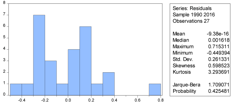
   Figure 1:

   Normality Test
   
   
   

1. 

   Figure Options

   • View in workspace

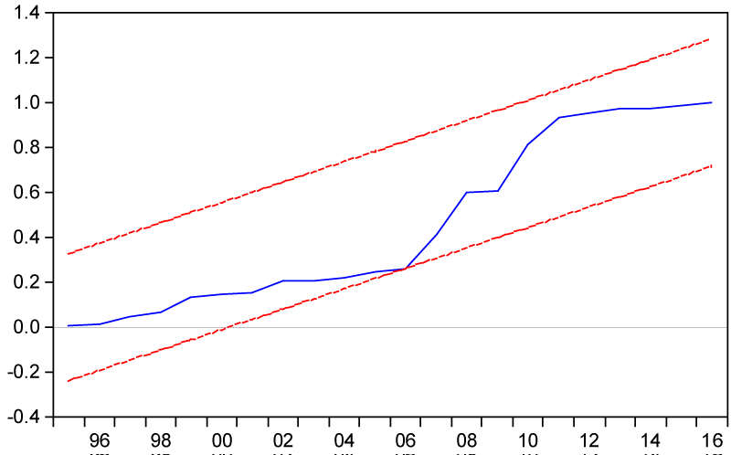
   Figure 2:

   CUSUMQ Test.
   
   
   

Conclusion / Recommendations

The role of agriculture in any economy is indeed significant and cannot be over-emphasized. It is one of the most dominant sectors in any economy as the very survival of every nation depends on how well or bad its agricultural sub-sector is managed. It is indeed not just a major source of livelihood for its citizens but a source of foreign exchange earner to the nation. This is because apart from providing food for the teeming population of the economy, it is the only source of raw materials that serves as input for other sectors in their production process. It is in recognition of this pivotal role played by the agricultural sector of the economy that this study becomes imperative. The main object of the study is to investigate the effect of Agricultural input on Agricultural productivity in Nigeria from 1990 to 2016 using secondary annual time series data sourced from World Bank database [1], and Central Bank of Nigeria Statistical Bulletin [13]. The methodology adopted for the study was first and foremost unit root test using Augmented Dickey-Fuller (ADF); a test for long-run relationship (Johansen cointegration), Granger causality test and then the Ordinary Least Squares (OLS) multiple regression method to determine the effect of the independent variables in the model on the dependent variable.

Variables in the model were both stationary as well as exhibited long-run equilibrium relationship. Empirical findings revealed that agricultural productivity has positive influence on government expenditure in the sector but not the other way round. This finding is in line with the earlier OLS regression result of an inverse relationship between government expenditure and agricultural output. It further negates the formulated hypothesis in section one of this study that “there is no causality relationship between government expenditure on agriculture and agricultural output”. Since empirical findings supports hypotheses earlier formulated for this study, it is thus concluded that government spending in agricultural sector does not contribute to positive increases in output from the sector. Secondly, agricultural machinery has no significant effect on agricultural productivity in Nigeria and finally, agricultural credit has no significant impact on agricultural productivity in Nigeria between 1990 to 2016.

This study thus aligns with the work of Ajie, Ojiya & Mamman [14], that successive administrations in Nigeria has not seen reason to come close to fulfilling internationally benchmarked budgetary recommendations for the agricultural sector since her independence. This is a disturbing trend. While sister African countries like Ivory Coast, Ghana and Ethiopia dedicates a larger percentage of their budget to the agricultural sub-sector, Nigeria with a spiraling population of over 180 million mouths to feed has displayed a carefree attitude towards recommendations from international agencies on the need to give priority to the sector in terms of funding. A country’s future in terms of food security is a function of government’s commitment to making its agriculture work, and working, very effectively and efficiently towards delivering expected dividends.

The following is therefore recommended for policy implementation:

(a) If the Nigeria government really want to attain the objective of self-sufficiency in food production, the government need to put in place policy and modalities that will encourage existing banks (both commercial and agricultural banks) to make credit facilities readily available to farmers with personnel assigned to monitor and ensure that such funds are judiciously used for the purpose which it is taken.

(b) Furthermore, government must provide funds to acquire sophisticated farm tools (harvesters, tractors, herbicides, fertilizer etc) and as well build irrigation, dams, storage facilities and establish food processing industries across the country to enable farmers increase productivity, process and preserve their food stuff.

(c) Finally, government spending on agricultural sector must of a necessity be increased. Similarly, the present lackluster and uninspiring attitude of government to management of appropriated funds must also change. Corrupt civil servants, contractors and bureaucrats who divert and misappropriate allocated funds for the growth of the sector must be punished to serve as deterrent to other intending treasury looters. The various financial crimes commissions such as EFCC and ICPC should be strengthened to do this.